Gravity Anomaly Over a Buried Point Mass

Previously we defined the gravitational acceleration due to a point mass as

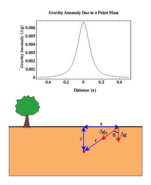
where g is the gravitational constant, m is the mass of the point mass, and r is the distance between the point mass and our observation point. The figure below shows the gravitational acceleration we would observe over a buried point mass. Notice, the acceleration is highest directly above the point mass and decreases as we move away from it.

Computing the observed acceleration based on the equation given above is easy and instructive. First, let's derive the equation used to generate the graph shown above. Let z be the depth of burial of the point mass and x is the horizontal distance between the point mass and our observation point. Notice that the gravitational acceleration caused by the point mass is in the direction of the point mass; that is, it's along the vector r. Before taking a reading, gravity meters are leveled so that they only measure the vertical component of gravity; that is, we only measure that portion of the gravitational acceleration caused by the point mass acting in a direction pointing down. The vertical component of the gravitational acceleration caused by the point mass can be written in terms of the angle as

Now, it is inconvenient to have to compute r and for various values of x before we can compute the gravitational acceleration. Let's now rewrite the above expression in a form that makes it easy to compute the gravitational acceleration as a function of horizontal distance x rather than the distance between the point mass and the observation point r and the angle .

can be written in terms of z and r using the trigonometric relationship between the cosine of an angle and the lengths of the hypotenuse and the adjacent side of the triangle formed by the angle.

Likewise, r can be written in terms of x and z using the relationship between the length of the hypotenuse of a triangle and the lengths of the two other sides known as Pythagorean Theorem.

Substituting these into our expression for the vertical component of the gravitational acceleration caused by a point mass, we obtain

Knowing the depth of burial, z, of the point mass, its mass, m, and the gravitational constant, G, we can compute the gravitational acceleration we would observe over a point mass at various distances by simply varying x in the above expression. An example of the shape of the gravity anomaly we would observe over a single point mass is shown above.

Therefore, if we thought our observed gravity anomaly was generated by a mass distribution within the earth that approximated a point mass, we could use the above expression to generate predicted gravity anomalies for given point mass depths and masses and determine the point mass depth and mass by matching the observations with those predicted from our model.

Although a point mass doesn't appear to be a geologically plausible density distribution, as we will show next, this simple expression for the gravitational acceleration forms the basis by which gravity anomalies over any more complicated density distribution within the earth can be computed.

❮❮ Previous Next ❯❯