Local/Regional Gravity Anomaly Separation Example

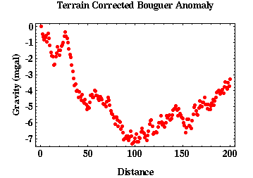
As an example of estimating the regional anomaly from the recorded data and isolating the local anomaly with this estimate consider using a moving average operator. With this technique, an estimate of the regional gravity anomaly at some point along a profile is determined by averaging the recorded gravity values at several nearby points. The number of points over which the average is calculated is referred to as the length of the operator and is chosen by the data processor. Averaging gravity values over several observation points enhances the long-wavelength contributions to the recorded gravity field while suppressing the shorter-wavelength contributions. Consider the sample gravity data shown below.

Moving averages can be computed across this data set. To do this the data processor chooses the length of the moving average operator. That is, the processor decides to compute the average over 3, 5, 7, 15, or 51 adjacent points. As you would expect, the resulting estimate of the regional gravity anomaly, and thus the local gravity anomaly, is critically dependent on this choice. Shown below are two estimates of the regional gravity anomaly using moving average operators of lengths 15 and 35.

Depending on the features of the gravity profile the processor wishes to extract, either of these operators may be appropriate. If we believe, for example, the gravity peak located at a distance of about 30 on the profile is a feature related to a local gravity anomaly, notice that the 15 length operator is not long enough. The average using this operator length almost tracks the raw data, thus when we subtract the averages from the raw data to isolate the local gravity anomaly the resulting value will be near zero. The 35 length operator, on the other hand, is long enough to average out the anomaly of interest, thus isolating it when we subtract the moving average estimate of the regional from the raw observations.

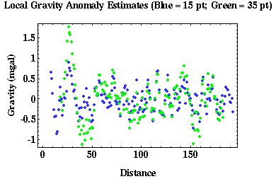
The residual gravity estimates computed for each moving average operator are shown below.

As expected, few interpretable anomalies exist after applying the 15 point operator. The peak at a distance of 30 has been greatly reduced in amplitude and other short-wavelength anomalies apparent in the original data have been effectively removed. Using the 35 length operator, the peak at a distance of 30 has been successfully isolated and other short-wavelength anomalies have been enhanced. Data processors and interpreters are free to choose the operator length they wish to apply to the data. This choice is based solely on the features they believe represent the local anomalies of interest. Thus, separation of the regional from the local gravity field is an interpretive process.

Although the interpretive nature of the moving average method for estimating the regional gravity contribution is readily apparent, you should be aware that all of the methods described on the previous page require interpreter input of one form or another. Thus, no matter which method is used to estimate the regional component of the gravity field, it should always be considered an interpretational process.

❮❮ Previous Next ❯❯