Tidal and Drift Corrections: Data Reduction

Using observations collected by the looping field procedure, it is relatively straight forward to correct these observations for instrument drift and tidal effects. The basis for these corrections will be the use of linear interpolation to generate a prediction of what the time-varying component of the gravity field should look like. Shown below is a reproduction of the spreadsheet used to reduce the observations collected in the survey defined on the last page.

The first three columns of the spreadsheet present the raw field observations; column 1 is simply the daily reading number (that is, this is the first, second, or fifth gravity reading of the day), column 2 lists the time of day that the reading was made (times listed to the nearest minute are sufficient), column 3 represents the raw instrument reading (although an instrument scale factor needs to be applied to convert this to relative gravity, and we will assume this scale factor is one in this example).

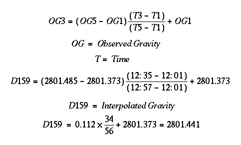
A plot of the raw gravity observations versus survey station number is shown above. Notice that there are three readings at station 9625. This is the base station which was occupied three times. Although the location of the base station is fixed, the observed gravity value at the base station each time it was reoccupied was different. Thus, there is a time varying component to the observed gravity field. To compute the time-varying component of the gravity field , we will use linear interpolation between subsequent reoccupations of the base station. For example, the value of the temporally varying component of the gravity field at the time we occupied station 159 (dark gray line) is computed using the expressions given below.

After applying corrections like these to all of the stations, the temporally corrected gravity observations are plotted below.

There are several things to note about the corrections and the corrected observations.

• One check to make sure that the corrections have been applied correctly is to look at the gravity observed at the base station. After application of the corrections, all of the gravity readings at the base station should all be zero.
• The uncorrected observations show a trend of increasing gravitational acceleration toward higher station number. After correction, this trend no longer exists. The apparent trend in the uncorrected observations is a result of tides and instrument drift.

❮❮ Previous Next ❯❯